15-418 Final Project Report

Bromide -- Fast CNN Inference In Halide

back to project index

github

Summary

We have implemented a general Convolutional Neural Networks inference program using the Halide image processing language which is scheduled to be fast(-er than Caffe, up to 3x) on a single machine using CPU.

Why we did this (Background)

CNN

Lots of modern-day machine learning applications, such as AlphaGo, are using Convolutional Neural Networks (CNNs) for classification tasks. Therefore, the performance of training and inference with CNNs is fairly important. For huge data sets and large CNN configurations, training can take several days, making it meaningful to speed up the training process. Besides, in real-time applications, such as Apple Siri, the time spent in inference is also expected to be short, so that the delay will be tolerable or more satisfactory for users.

For testing purpose, we are using MNIST (a database of handwritten digits and we use a typical CNN, LeNet to perform inference on it) and AlexNet(which is designed to do classification towards ImageNet).

The structure of LeNet is illustrated as below:

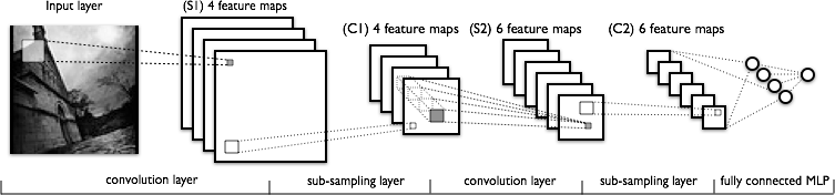
The LeNet that we use is mainly composed of the following layers by order: conv, pooling, conv, pooling, fully-connected, relu, fully-connected, softmax.

The structure of AlexNet is illustrated as below:

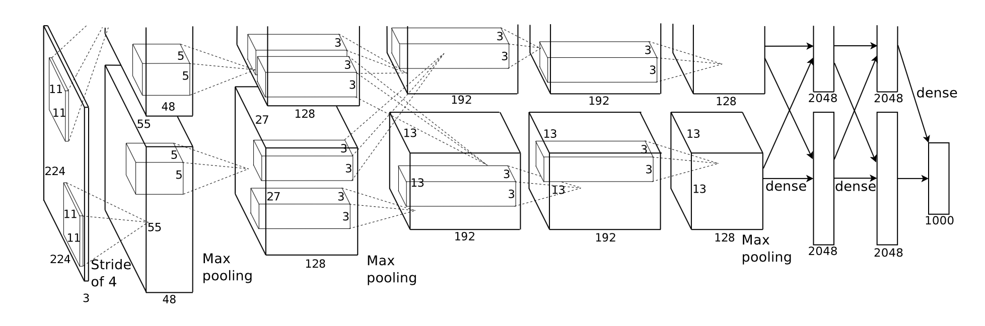
The AlexNet that we use is mainly composed of the following layers by order: conv, relu, norm, pooling, conv, relu, norm, pooling, conv, relu, conv, relu, conv, relu, pooling, fully-connected, relu, drop, fully-connected, relu, drop, fully-connected, softmax.

Caffe

Caffe is a deep learning framework currently widely used to both train and test CNN. It is known for its speed, modularity and clear expressions and settings of networks and relevant processes. In our project, Caffe is selected to be a benchmark for us to compete against in terms of speed.

Halide

Halide is a language and compiler for optimizing parallelism,locality, and re-computation in image processing pipelines. Since it provides many scheduling interfaces to handle matrices, it is a great source for CNN implementation, where the intermediate results are also matrices. Therefore, by carefully scheduling CNN training and inference with Halide, an obvious speedup is expected.

What we did (Results)

We have implemented this inference program which is tested towards MNIST (LeNet) and AlexNet (ImageNet), and it is compared against Caffe (testing of the network). Luckily, we have achieved better performance than Caffe in our limited tested scenarios. The following figures and data generally use Caffe as their counterpart for comparison. Our implementation is referred to as "bromide".

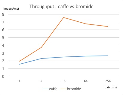
The throughput of LeNet is illustrated as below:

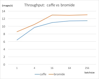
The throughput of AlexNet is illustrated as below:

The latency of LeNet and AlexNet is illustrated as below: (latency here stands for the time to perform inference on a single input image, the smaller the better)

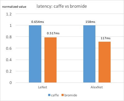
As we can see from the figures above, for the batchsize 16 of LeNet, the speedup (in terms of throughput) of Bromide over Caffe is roughly 3.04x, and the average latency is 21% (LeNet) and 26% (AlexNet) better than Caffe. Although these are not very significant, the results surely give us some hope in the power of scheduling in Halide.

Experimental setup:

Input (LeNet): 28x28x1
Input (AlexNet): 227x227x3
Output: label/classification of the picture. We actually stopped after the last layer (softmax) because choosing the most likely label is irrelevant with the performance, so this part is cut after we tested the correctness of the network)
Machine: all of these tests are conducted on a machine that has 2 processors (Intel(R) Core(TM) i7-4790 CPU @ 3.60GHz). This kind of CPU has 4 cores and 8 thereads, with 8MB cache size.
Batch size: batch size stands for the number of images for one batch of input. It ranges from 1 to 256, so we have a good observation of the change of performance.

Profile of runtime:

This is the profile for a run of batch size 64 on AlexNet (We ommitted the items with roughly 0% time):

Layer	Time(ms)	%
conv	436.2	8
constant_exterior	375.8	7
norm	135.9	2
sum#1	114.9	2
conv	502.1	10
constant_exterior	348.2	7
norm	88.5	1
sum#2	71.7	1
conv	266.3	5
constant_exterior	280.0	5
conv	409.5	8
constant_exterior	467.2	9
conv	342.5	6
constant_exterior	284.0	5
sum#3(fully)	492.6	9
sum#4(fully)	100.52	2
sum#6(fully)	207.2	4

conv: convolutional layer. norm: normalization layer. constant_exterior & sum: some halide built-in functions. The last fully-connected layers spent most of their time on sum().

We can tell that most time-consuming layers, as we expected, is convolutional layers and fully connected layers. constant_exterior mostly take place in convolution layers and the last 3 sum functions are in fully-connected layers. Therefore, what we can do is to further tune the convolutional layer and fully connected layer. One thing we noticed when we compared to Caffe is that, our convolutional layer outperforms Caffe a lot, while Caffe's fully-connected layer performs better than Bromide's. This is not unexpected, because there is still a lot to do in the scheduling of fully-connected layer. If we can futher reduce the time there (getting rid of sum() reduction and performing more fine-tuning), the performance of bromide would be a lot more desirable.

How we did it (A: Methodology)

Usually, when we implement a CNN, we would like to build it layer by layer. One problem lying here is that every time we transmit the intermidiate results from one layer to its successor layer, we need to do a read and a write.

This seems natural, but sometimes unnecessary. Take activation layer as an example, it's doing per-element computation, such as applying a ReLU function to all elements in the intermediate maps. Actually, this procedure can be embedded in the either the previous layer or the next layer, to avoid a read and a write. This loop-fusion method can be easily impelemented using Halide.

Another thing worth noting is that the proper use of L3 cache can greatly increase the performance. When the data need to be reused, we can benefit from letting the data sit in the cache and wait for being called next time. Convolution layer, pooling layer, normalization layer and fully-connected layer are probably involved with data reuse. Therefore, tiling the maps can be a reasonable way.

Also, we made an effort to make good use of SIMD and multi-threading techniques, based on their different characteristics. When using SIMD, we hope there's less divergence. Fortunately, most of the computations in CNN don't include braches. Therefore, we can use SIMD either in the inner loop or the outer loop. Since multi-threading and scheduling were to take place, we performed vectorization in the inner loop. When using multi-threading, we hope there's less synchronization. We chose to do multi-threading on the outermost loop(s) in Bromide and it turns out to be a good choice. Also, we note that the total number of threads in a machine is far less than the actual parallelizable units. To reduce synchronization, it's better to put multi-threading at the outer loop of the embedded loops.

Furthermore, other scheduling approaches, such as tiling, unrolling, and reordering, are applied here, depending on the specific layers and map sizes. It took us a great amount of time to tune the scheduling for the layers (mainly convolutional layers).

Hints from Caffe

We actually profiled Caffe to try to get some hints to perform our optimization. This is an example of batch size 64 on AlexNet:

Layer	Time(ms)
conv1	671.791
relu1	14.302
norm1	529.359
pool1	56.879
conv2	1246.95
relu2	9.052
norm2	343.957
pool2	39.369
conv3	1022.71
relu3	3.168
conv4	791.008
relu4	3.296
conv5	542.841
relu5	2.103
pool5	9.796
fully-connected6	196.115
relu6	0.202
drop6	1.854
fully-connected7	86.68
relu7	0.203
drop7	1.857
fully-connected8	21.642

As we can tell from the table, most of the time are spent on convolutional layers. Caffe transformed convolution into matrix multiplication, where it can make use of well-tuned implementations like Intel's MKL to accelerate the speed. However, we think this can be improved since Caffe's method will generate a lot of memory traffic and do a lot of redundat. Therefore, performing well-tuned scheduling based on the definition of convolution might give us speedup, which is the most significant part of our implementation.

How we did it (B: Details)

We would introduce the details of the implementation (majorly scheduling) by each layer. Flatten layer, activation layer and drop layer are fairly straightforward thus we would mainly discuss other layers about their scheduling.

Basic Settings

Every layer has a member called cnnff, standing for the collection of the feedforward values. It generally has 4 dimensions, (x, y, z, w), corresponding to the column-index, row-index, map-index (3rd dimension), and batch size. All those layers are written in separate files and they are welded in the main function to build networks for testing. Scheduling is performed inside the layers.

Kernels of convolution are traversed using Halide::RDom, which is denoted as dom in our program and used to construct a multi-dimensional reduction domain. If the kernel has 3 dimensions, it will be denoted by dom.x, dom.y, dom.z.

Input Layer

We process the input data (trained weights) using a similar way to Caffe. The model (bvlc_alexnet.caffemodel) and mean (imagenet_mean.inarayproto) are parsed based on the functions provided by Caffe responsible for translating files using Protocol Buffer.

Convolutional Layer

Version 1:

conv_basic(x, y, z, w) = Halide::sum(last_layer.cnnff(x + dom.x, y + dom.y, dom.z + group_idx * input_group_size, w) * kernels(dom.x, dom.y, dom.z, map_idx + group_idx * group_size) + bias(z));

We are mainly doing intuitive implementation as well as using Halide::sum() and Func.ompute_root() in version 1. In convolutional layer, each pixel of an output map is computed according to the definition as the weighted sum of a filter window.

The Halide::sum() function is used for inline reduction over the given domain (in this case, the domain would be 3-d, corresponding to the filter window of convolution). Func.compute_root() in Halide is used to compute the Func ahead of the following program (Funcs will be combined inline in Halide if there is no functions like compute_root() or compute_at() to explicitly order it to perform computation to the point). Func is a Halide class standing for a pipleline stage, which is a pure function that defines what value each pixel should have, similar to a computed image.

Version 2:

input_ = Halide::BoundaryConditions::constant_exterior(last_layer.cnnff, 0, 0, last_layer.size[0], 0, last_layer.size[1]);
cnnff(x, y, z, w) = bias(z);
cnnff(x, y, z, w) += kernels(dom.x, dom.y, dom.z, z) * input_(x * stride_x + dom.x - pad_x, y * stride_y + dom.y - pad_y, dom.z, w);
cnnff.update().split(y, y_outer, y_inner, y_size).split(z, z_outer, z_inner, z_size);
cnnff.update().reorder(y_inner, z_inner, y_outer, dom.z, z_outer).vectorize(x, 8);
cnnff.update().parallel(w);
cnnff.update().unroll(dom.x).unroll(dom.y);
input_.compute_at(cnnff, z_inner);

Convolution layer is a meaningful implementation exploiting the power of scheduling in Halide. We basically split y and z and reorder to get a tile, in order to find a point that reaches a good balance of memory traffic and locality which leads to a good performance. A typical tile would be loop over (from inner to outer) y_inner, y_outer, z_inner, z_outer, however, reordering the domain loop dom.z before (y_outer or) z_outer would led to a elevation of performance because of more locality. Vectorization, parallelism and unrolling were performed here as well. It is fairly intuitive to vectorize over the innermost variable (x) of cnnff and parallelize the outermost one. This is tested as well, we noticed a performance drop if on other layers. Unrolling is performed at two innermost domain variables (dom.x and dom.y) since they have a typically small range, which is the same reason why we did not put vectorization onto dom.x or dom.y. The compute_at(func, var) function performs computation of func for every unique value of var, which would enable us to compute the block of inner loop variables (y_inner and z_inner) to actually instantiate the above scheduling and increase data locality and reduce redundant calculation. y_size and z_size are 2 parameters to tune towards the tile scheduling. They varies on different networks and different machines. On our settings, a good value would be 32 for both.

Fully Connected Layer

Halide::RDom dom(0, last_layer.size[0]);
cnnff(x, y, z, w) = Halide::sum(last_layer.cnnff(dom.x, y, z, w) * weights(dom.x, x)) + bias(x);
cnnff.parallel(w);
cnnff.vectorize(x, 8);
cnnff.compute_root();

Fully connected layer is basically a matrix multiplication. If the batch size is equal to 1, it's a matrix multiplied by a vector. Otherwise, it's a multiplication between two matrices. A lot of the optimization/scheduling methods can be used here. Note that for the multiplication between a matrix and a vector, there's data reuse only in terms of the vector, but no data reuse for matrix. So a reasonable scheduling is row-by-row multiplication between matrix and vector. However, for the multiplication between two matrices, more sophisticated methods should be considered. In this project, we tried tiling the matrices into blocks, and tuning the block size to let it fit in the L3 cache. But we found that in our experiments, similarly good perforamnce can be achieved by the straighforward impelmentation of matrix multiplication.

Also, for both matrix-vector multiplication and matrix-matrix multiplication, we make use of SIMD and multi-threading implementation. We schedule them in different dimensions so that they can work together with less synchronization. We use multi-threading for the "batch" dimension, referring to any test image. And we use SIMD for each image. To compute each pixel, there's a inner-product between vectors. This procedure is done by the reduction function sum() built in Halide.

Pooling Layer

Halide::Func sub_maps("sub_maps");
Halide::RDom dom(0, pool_x, 0, pool_y);
if(pool_func == "max") {
   sub_maps(x, y, z, w) = Halide::maximum(last_layer.cnnff(x + dom.x, y + dom.y, z, w));
}else if(pool_func == "average") {
   sub_maps(x, y, z, w) = Halide::sum(last_layer.cnnff(x + dom.x, y + dom.y, z, w)) / (pool_x * pool_y);
}
cnnff(x, y, z, w) = sub_maps(x * stride_x - pad_x, y * stride_y - pad_y, z, w);
cnnff.vectorize(x, 8);
cnnff.compute_root();

Pooling layer is similar to the convolution layer, in that there is a window that traverses the maps, and performs reduction at each time. Therefore, similar optimization (similar to the above) can be used in pooling.

But we also notice that, pooling doesn't take a large proportion in the overall latency. Therefore, we simply used the built-in reduction function max, and vectorized it by SIMD. We didn't choose to use multi-threading, because the overhead is not worthwhile. In our observation, pooling layer of bromide can achieve 10x speedup compared to caffe implementation.

Further Analysis of Implementation

General Challenges

Halide is a language targeted at image processing, which provides a set of computation scheduling methods to help programmers exploit data locality and achieve higher performance when writing parallel programs. However, since it is not designed for deep learning methods, it does not have intrinsic support for the typical computation patterns or algorithms in deep learning, for example, convolution.

 Nowadays there are many a mature (sort of) implementation of deep learning methods.

For example, Caffe, is a frequently seen framework in the world of deep neural networks. One feature about Caffe is that it takes advantage of a fast matrix multiplication library like Intel's MKL when running convolutional neural networks by using matrix multiplications. However, breaking down the convolutional layers to matrix multiplications might not produce a desirable performance speedup since Halide does not natively support matrix multiplication. We thought of using FFT could avoid both the original complex convolution computations and the need for fast matrix multiplication. Although doing the DFT and its inverse will take some time but this might be better than the matrix multiplications way. Anyway, we think doing Fourier transform only makes sense when the weight has one or more huge dimesion(s), so the target that we aim here is to schedule and tune the program using Halide to achieve admissible performance on CPU or GPU. This really turned out to be tough.

 It is not easy to understand all the scheduling capabilities provided by Halide. Although the syntax and configurations are made very intuitive and powerful, the conciseness takes a lot of effort to grasp the scheduling. It took us a lot of time to understand and test in terms of making tradeoff between memory bandwidth (locality), parallelism and doing redundant work, which are made more explicit by Halide.

Analysis of Implementation

One limitation of our speedup is that it is difficult to make the "best" trade-off between redundant computation and memory accesses. If we make more synchronizations for the intermediate layers, more memory accesses will occur because we have to store the intermediate results and load these results later. However, if we make less synchronizations, we will probably do much redundant computation works. Therefore, a better trade-off between redundant computation and memory accesses has to be made in order to reduce latency. This trade-off is decided by how we schedule, such as split, reorder and fuse our loops. For example, the size of tiles are being heavily tested in our implementation. For example, a major drop takes place if the sizes of our tile in convolutional layers grow to be larger than the size of cache.

In our CNN implementations, synchronization is made by "compute_root() or compute_at()". The intermediate results for a Func will be stored only when we schedule this Func with compute_root(). We basically set compute_root() for the Funcs that compute each output pixels with multiple pixels and parameters. But a more careful tuning here may help further increase the speed. At first we performed no compute_root on every layer, which results in a full inline version of CNN, leading to a performance of more than 200x slower than Caffe. However, it is not necessary to put compute_at() in every layer or put compute_at() at many dimensions. Doing too much stage synchronization would hurt the performance significantly as well. For example, applying compute_root() at every layer would lead to a 2~5x slower version of our code. We need to try to test more on this part in order to improve the performance.

Within each Func, we paralleled with multi-threading and SIMD on different levels. We put the multi-threading at the outer loop to decrease the proportion of the scheduling overhead. And we use SIMD in the innermost loop of cnnff to reduce divergence, as well as make better use of locality. Also, we split the maps and reorder the for loops, to further deploy the locality. The implementation does not lack parallelism, but there might be some potential to better schedule the computation to fit the computating and memory resources of different machines and settings. The choice of levels to perform parallelism influences the performance to a great degree. For example, if we change the vectorization from x to higher or lower in the convolutional layer, we would notice a significant drop of performance as much as 3x. If we fuse z_outer and w in convolutional layer to do multi-threading, it does not change the performance but if we reorder the loops, such as reorder z_outer to be the outermost, the performance is hurt badly. This choice might limit our performance because we might not choose the best order and level of parallelism up to this point.

The different setups of CNNs has some influence on the performance of our implementation as well. For example, different sizes of convolution kernel would affect the performance of our choice of parallelism. If one dimension of the kernel size is bigger than the number of SIMD lanes, it might be better to do vectorization on the domain variables (dom.x and dom.y) rather than x. There is nothing like a best set of parameters and schedule for every network, but it is possible to find a generally better solution to some frequently used CNNs as LeNet and AlexNet. We need to admit that the variety of networks pose a difficulty and limitation on our elevation of performance.

Room of Elevation

As we can tell from the two tables of profiling Caffe and Bromide's runtime on AlexNet with a batchsize 64, we significantly outperformed Caffe on convolutional layers but did bad on fully-connected layers. This is because we did not manage to get a nicely tuned scheduling of this layer up to now. Although in fully-connected layers, if using matrix multiplication, we no longer need to do so much copying and redundant work as in convolutional layers, which can better take the advantage of fine-tuned matrix multiplication, we still think it might be feasible to get the same or even better performance on this layer than Caffe if we can tune the schedule better and given that Halide provides a lot of optimization under the scheduling. Elevation of the performance of Bromide on fully-connected layers to the same level of Caffe would enable Bromide to have a much better general performance.

Besides, the tuning of convolutional layers is not perfect. Using the current strategy, we think there is still a lot of space to explore, for example we could go with different tile size with different order of loops. Tuning these parameters towards the specification of the machine would further bring up the performance.

Future Work

Our future work will also include allowing the program to adaptively select a close to best scheduling strategy for each network and machine type. Currently, we have to differentiate the details of scheduling for LeNet and AlexNet, such as tiling and reordering. However, it would be a great step if the scheduling stategy can be automatically created for each application.

References

Work Divided

Roughly equal work by each student.

References

- Halide source code: https://github.com/halide/Halide.
- Ragan-Kelley, J., Barnes, C., Adams, A., Paris, S., Durand, F. and Amarasinghe, S., 2013. Halide: a language and compiler for optimizing parallelism, locality, and recomputation in image processing pipelines. ACM SIGPLAN Notices, 48(6), pp.519-530.
- Krizhevsky, Alex, Ilya Sutskever, and Geoffrey E. Hinton. "Imagenet classification with deep convolutional neural networks." Advances in neural information processing systems. 2012.
- LeCun, Yann, et al. "Comparison of learning algorithms for handwritten digit recognition." International conference on artificial neural networks. Vol. 60. 1995.